Egftnjytyk

In physics and fluid mechanics, a boundary layer is an important concept and refers to the layer of fluid in the immediate vicinity of a bounding surface where the effects of viscosity are significant.

In the Earth's atmosphere, the atmospheric boundary layer is the air layer near the ground affected by diurnal heat, moisture or momentum transfer to or from the surface. On an aircraft wing the boundary layer is the part of the flow close to the wing, where viscous forces distort the surrounding non-viscous flow.

Types of boundary layer

Boundary layer visualization, showing transition from laminar to turbulent condition

Laminar boundary layers can be loosely classified according to their structure and the circumstances under which they are created. The thin shear layer which develops on an oscillating body is an example of a Stokes boundary layer, while the Blasius boundary layer refers to the well-known similarity solution near an attached flat plate held in an oncoming unidirectional flow and Falkner–Skan boundary layer, a generalization of Blasius profile. When a fluid rotates and viscous forces are balanced by the Coriolis effect (rather than convective inertia), an Ekman layer forms. In the theory of heat transfer, a thermal boundary layer occurs. A surface can have multiple types of boundary layer simultaneously.

The viscous nature of airflow reduces the local velocities on a surface and is responsible for skin friction. The layer of air over the wing's surface that is slowed down or stopped by viscosity, is the boundary layer. There are two different types of boundary layer flow: laminar and turbulent.^[1]

Laminar Boundary Layer Flow

The laminar boundary is a very smooth flow, while the turbulent boundary layer contains swirls or "eddies." The laminar flow creates less skin friction drag than the turbulent flow, but is less stable. Boundary layer flow over a wing surface begins as a smooth laminar flow. As the flow continues back from the leading edge, the laminar boundary layer increases in thickness.

Turbulent Boundary Layer Flow

At some distance back from the leading edge, the smooth laminar flow breaks down and transitions to a turbulent flow. From a drag standpoint, it is advisable to have the transition from laminar to turbulent flow as far aft on the wing as possible, or have a large amount of the wing surface within the laminar portion of the boundary layer. The low energy laminar flow, however, tends to break down more suddenly than the turbulent layer.

Aerodynamics

Ludwig Prandtl

Laminar boundary layer velocity profile

The aerodynamic boundary layer was first defined by Ludwig Prandtl in a paper presented on August 12, 1904 at the third International Congress of Mathematicians in Heidelberg, Germany. It simplifies the equations of fluid flow by dividing the flow field into two areas: one inside the boundary layer, dominated by viscosity and creating the majority of drag experienced by the boundary body; and one outside the boundary layer, where viscosity can be neglected without significant effects on the solution. This allows a closed-form solution for the flow in both areas, a significant simplification of the full Navier–Stokes equations. The majority of the heat transfer to and from a body also takes place within the boundary layer, again allowing the equations to be simplified in the flow field outside the boundary layer. The pressure distribution throughout the boundary layer in the direction normal to the surface (such as an airfoil) remains constant throughout the boundary layer, and is the same as on the surface itself.

The thickness of the velocity boundary layer is normally defined as the distance from the solid body to the point at which the viscous flow velocity is 99% of the freestream velocity (the surface velocity of an inviscid flow). Displacement thickness is an alternative definition stating that the boundary layer represents a deficit in mass flow compared to inviscid flow with slip at the wall. It is the distance by which the wall would have to be displaced in the inviscid case to give the same total mass flow as the viscous case. The no-slip condition requires the flow velocity at the surface of a solid object be zero and the fluid temperature be equal to the temperature of the surface. The flow velocity will then increase rapidly within the boundary layer, governed by the boundary layer equations, below.

The thermal boundary layer thickness is similarly the distance from the body at which the temperature is 99% of the freestream temperature. The ratio of the two thicknesses is governed by the Prandtl number. If the Prandtl number is 1, the two boundary layers are the same thickness. If the Prandtl number is greater than 1, the thermal boundary layer is thinner than the velocity boundary layer. If the Prandtl number is less than 1, which is the case for air at standard conditions, the thermal boundary layer is thicker than the velocity boundary layer.

In high-performance designs, such as gliders and commercial aircraft, much attention is paid to controlling the behavior of the boundary layer to minimize drag. Two effects have to be considered. First, the boundary layer adds to the effective thickness of the body, through the displacement thickness, hence increasing the pressure drag. Secondly, the shear forces at the surface of the wing create skin friction drag.

At high Reynolds numbers, typical of full-sized aircraft, it is desirable to have a laminar boundary layer. This results in a lower skin friction due to the characteristic velocity profile of laminar flow. However, the boundary layer inevitably thickens and becomes less stable as the flow develops along the body, and eventually becomes turbulent, the process known as boundary layer transition. One way of dealing with this problem is to suck the boundary layer away through a porous surface (see Boundary layer suction). This can reduce drag, but is usually impractical due to its mechanical complexity and the power required to move the air and dispose of it. Natural laminar flow techniques push the boundary layer transition aft by reshaping the airfoil or fuselage so that its thickest point is more aft and less thick. This reduces the velocities in the leading part and the same Reynolds number is achieved with a greater length.

At lower Reynolds numbers, such as those seen with model aircraft, it is relatively easy to maintain laminar flow. This gives low skin friction, which is desirable. However, the same velocity profile which gives the laminar boundary layer its low skin friction also causes it to be badly affected by adverse pressure gradients. As the pressure begins to recover over the rear part of the wing chord, a laminar boundary layer will tend to separate from the surface. Such flow separation causes a large increase in the pressure drag, since it greatly increases the effective size of the wing section. In these cases, it can be advantageous to deliberately trip the boundary layer into turbulence at a point prior to the location of laminar separation, using a turbulator. The fuller velocity profile of the turbulent boundary layer allows it to sustain the adverse pressure gradient without separating. Thus, although the skin friction is increased, overall drag is decreased. This is the principle behind the dimpling on golf balls, as well as vortex generators on aircraft. Special wing sections have also been designed which tailor the pressure recovery so laminar separation is reduced or even eliminated. This represents an optimum compromise between the pressure drag from flow separation and skin friction from induced turbulence.

When using half-models in wind tunnels, a peniche is sometimes used to reduce or eliminate the effect of the boundary layer.

Boundary layer equations

The deduction of the boundary layer equations was one of the most important advances in fluid dynamics. Using an order of magnitude analysis, the well-known governing Navier–Stokes equations of viscous fluid flow can be greatly simplified within the boundary layer. Notably, the characteristic of the partial differential equations (PDE) becomes parabolic, rather than the elliptical form of the full Navier–Stokes equations. This greatly simplifies the solution of the equations. By making the boundary layer approximation, the flow is divided into an inviscid portion (which is easy to solve by a number of methods) and the boundary layer, which is governed by an easier to solve PDE. The continuity and Navier–Stokes equations for a two-dimensional steady incompressible flow in Cartesian coordinates are given by

∂u∂x+∂υ∂y=0{displaystyle {partial u over partial x}+{partial upsilon over partial y}=0}

u∂u∂x+υ∂u∂y=−1ρ∂p∂x+ν(∂2u∂x2+∂2u∂y2){displaystyle u{partial u over partial x}+upsilon {partial u over partial y}=-{1 over rho }{partial p over partial x}+{nu }left({partial ^{2}u over partial x^{2}}+{partial ^{2}u over partial y^{2}}right)}

u∂υ∂x+υ∂υ∂y=−1ρ∂p∂y+ν(∂2υ∂x2+∂2υ∂y2){displaystyle u{partial upsilon over partial x}+upsilon {partial upsilon over partial y}=-{1 over rho }{partial p over partial y}+{nu }left({partial ^{2}upsilon over partial x^{2}}+{partial ^{2}upsilon over partial y^{2}}right)}

where u{displaystyle u} and υ{displaystyle upsilon } are the velocity components, ρ{displaystyle rho } is the density, p{displaystyle p} is the pressure, and ν{displaystyle nu } is the kinematic viscosity of the fluid at a point.

The approximation states that, for a sufficiently high Reynolds number the flow over a surface can be divided into an outer region of inviscid flow unaffected by viscosity (the majority of the flow), and a region close to the surface where viscosity is important (the boundary layer). Let u{displaystyle u} and υ{displaystyle upsilon } be streamwise and transverse (wall normal) velocities respectively inside the boundary layer. Using scale analysis, it can be shown that the above equations of motion reduce within the boundary layer to become

u∂u∂x+υ∂u∂y=−1ρ∂p∂x+ν∂2u∂y2{displaystyle u{partial u over partial x}+upsilon {partial u over partial y}=-{1 over rho }{partial p over partial x}+{nu }{partial ^{2}u over partial y^{2}}}

1ρ∂p∂y=0{displaystyle {1 over rho }{partial p over partial y}=0}

and if the fluid is incompressible (as liquids are under standard conditions):

∂u∂x+∂υ∂y=0{displaystyle {partial u over partial x}+{partial upsilon over partial y}=0}

The order of magnitude analysis assumes the streamwise length scale significantly larger than the transverse length scale inside the boundary layer. It follows that variations in properties in the streamwise direction are generally much lower than those in the wall normal direction. Apply this to the continuity equation shows that υ{displaystyle upsilon }, the wall normal velocity, is small compared with u{displaystyle u} the streamwise velocity.

Since the static pressure p{displaystyle p} is independent of y{displaystyle y}, then pressure at the edge of the boundary layer is the pressure throughout the boundary layer at a given streamwise position. The external pressure may be obtained through an application of Bernoulli's equation. Let U{displaystyle U} be the fluid velocity outside the boundary layer, where u{displaystyle u} and U{displaystyle U} are both parallel. This gives upon substituting for p{displaystyle p} the following result

u∂u∂x+υ∂u∂y=UdUdx+ν∂2u∂y2{displaystyle u{partial u over partial x}+upsilon {partial u over partial y}=U{frac {dU}{dx}}+{nu }{partial ^{2}u over partial y^{2}}}

For a flow in which the static pressure p{displaystyle p} also does not change in the direction of the flow

dpdx=0{displaystyle {frac {dp}{dx}}=0}

so U{displaystyle U} remains constant.

Therefore, the equation of motion simplifies to become

u∂u∂x+υ∂u∂y=ν∂2u∂y2{displaystyle u{partial u over partial x}+upsilon {partial u over partial y}={nu }{partial ^{2}u over partial y^{2}}}

These approximations are used in a variety of practical flow problems of scientific and engineering interest. The above analysis is for any instantaneous laminar or turbulent boundary layer, but is used mainly in laminar flow studies since the mean flow is also the instantaneous flow because there are no velocity fluctuations present. This simplified equation is a parabolic PDE and can be solved using a similarity solution often referred to as the Blasius boundary layer.

Prandtl's transposition theorem

Prandtl^[2] observed that from any solution u(x,y,t), v(x,y,t){displaystyle u(x,y,t), v(x,y,t)} which satisfies the boundary layer equations, further solution u∗(x,y,t), v∗(x,y,t){displaystyle u^{*}(x,y,t), v^{*}(x,y,t)}, which is also satisfying the boundary layer equations, can be constructed by writing

u∗(x,y,t)=u(x,y+f(x),t),v∗(x,y,t)=v(x,y+f(x),t)−f′(x)u(x,y+f(x),t){displaystyle u^{*}(x,y,t)=u(x,y+f(x),t),quad v^{*}(x,y,t)=v(x,y+f(x),t)-f'(x)u(x,y+f(x),t)}

where f(x){displaystyle f(x)} is arbitrary. Since the solution is not unique from mathematical perspective,^[3] to the solution can added any one of an infinite set of eigenfunctions as shown by Stewartson^[4] and Paul A. Libby.^[5][6]

Von Kármán Momentum integral

von Kármán^[7] derived the integral equation by integrating the boundary layer equation across the boundary layer in 1921. The equation is

τwρU2=1U2∂∂t(Uδ1)+∂δ2∂x+2δ2+δ1U∂U∂x+vwU{displaystyle {frac {tau _{w}}{rho U^{2}}}={frac {1}{U^{2}}}{frac {partial }{partial t}}(Udelta _{1})+{frac {partial delta _{2}}{partial x}}+{frac {2delta _{2}+delta _{1}}{U}}{frac {partial U}{partial x}}+{frac {v_{w}}{U}}}

where

τw=μ(∂u∂y)y=0,vw=v(x,0,t),δ1=∫0∞(1−uU)dy,δ2=∫0∞uU(1−uU)dy{displaystyle tau _{w}=mu left({frac {partial u}{partial y}}right)_{y=0},quad v_{w}=v(x,0,t),quad delta _{1}=int _{0}^{infty }left(1-{frac {u}{U}}right)dy,quad delta _{2}=int _{0}^{infty }{frac {u}{U}}left(1-{frac {u}{U}}right)dy}

τw{displaystyle tau _{w}} is the wall shear stress, vw{displaystyle v_{w}} is the suction/injection velocity at the wall, δ1{displaystyle delta _{1}} is the displacement thickness and δ2{displaystyle delta _{2}} is the momentum thickness. Kármán-Pohlhausen Approximation is derived from this equation.

Energy integral

The energy integral was derived by Wieghardt.^[8][9]

2ερU3=1U∂∂t(δ1+δ2)+2δ2U2∂U∂t+1U3∂∂x(U3δ3)+vwU{displaystyle {frac {2varepsilon }{rho U^{3}}}={frac {1}{U}}{frac {partial }{partial t}}(delta _{1}+delta _{2})+{frac {2delta _{2}}{U^{2}}}{frac {partial U}{partial t}}+{frac {1}{U^{3}}}{frac {partial }{partial x}}(U^{3}delta _{3})+{frac {v_{w}}{U}}}

where

ε=∫0∞μ(∂u∂y)2dy,δ3=∫0∞uU(1−u2U2)dy{displaystyle varepsilon =int _{0}^{infty }mu left({frac {partial u}{partial y}}right)^{2}dy,quad delta _{3}=int _{0}^{infty }{frac {u}{U}}left(1-{frac {u^{2}}{U^{2}}}right)dy}

ε{displaystyle varepsilon } is the energy dissipation rate due to viscosity across the boundary layer and δ3{displaystyle delta _{3}} is the energy thickness.^[10]

Von Mises transformation

For steady two-dimensional boundary layers, von Mises^[11] introduced a transformation which takes x{displaystyle x} and ψ{displaystyle psi }(stream function) as independent variables instead of x{displaystyle x} and y{displaystyle y} and uses a dependent variable χ=U2−u2{displaystyle chi =U^{2}-u^{2}} instead of u{displaystyle u}. The boundary layer equation then become

∂χ∂x=νU2−χ∂2χ∂ψ2{displaystyle {frac {partial chi }{partial x}}=nu {sqrt {U^{2}-chi }}{frac {partial ^{2}chi }{partial psi ^{2}}}}

The original variables are recovered from

y=∫U2−χdψ,u=U2−χ,v=u∫∂∂x(1u)dψ.{displaystyle y=int {sqrt {U^{2}-chi }}dpsi ,quad u={sqrt {U^{2}-chi }},quad v=uint {frac {partial }{partial x}}left({frac {1}{u}}right)dpsi .}

This transformation is later extended to compressible boundary layer by von Kármán and HS Tsien.^[12]

Crocco's transformation

For steady two-dimensional compressible boundary layer, Luigi Crocco^[13] introduced a transformation which takes x{displaystyle x} and u{displaystyle u} as independent variables instead of x{displaystyle x} and y{displaystyle y} and uses a dependent variable τ=μ∂u/∂y{displaystyle tau =mu partial u/partial y}(shear stress) instead of u{displaystyle u}. The boundary layer equation then become

μρu∂∂x(1τ)+∂2τ∂u2−μdpdx∂∂u(1τ)=0{displaystyle mu rho u{frac {partial }{partial x}}left({frac {1}{tau }}right)+{frac {partial ^{2}tau }{partial u^{2}}}-mu {frac {dp}{dx}}{frac {partial }{partial u}}left({frac {1}{tau }}right)=0}

if dpdx=0,μρτ2∂τ∂x=1u∂2τ∂u2{displaystyle {text{if}} {frac {dp}{dx}}=0,quad {frac {mu rho }{tau ^{2}}}{frac {partial tau }{partial x}}={frac {1}{u}}{frac {partial ^{2}tau }{partial u^{2}}}}

The original coordinate is recovered from

y=μ∫duτ.{displaystyle y=mu int {frac {du}{tau }}.}

Turbulent boundary layers

The treatment of turbulent boundary layers is far more difficult due to the time-dependent variation of the flow properties. One of the most widely used techniques in which turbulent flows are tackled is to apply Reynolds decomposition. Here the instantaneous flow properties are decomposed into a mean and fluctuating component. Applying this technique to the boundary layer equations gives the full turbulent boundary layer equations not often given in literature:

∂u¯∂x+∂v¯∂y=0{displaystyle {partial {overline {u}} over partial x}+{partial {overline {v}} over partial y}=0}

u¯∂u¯∂x+v¯∂u¯∂y=−1ρ∂p¯∂x+ν(∂2u¯∂x2+∂2u¯∂y2)−∂∂y(u′v′¯)−∂∂x(u′2¯){displaystyle {overline {u}}{partial {overline {u}} over partial x}+{overline {v}}{partial {overline {u}} over partial y}=-{1 over rho }{partial {overline {p}} over partial x}+nu left({partial ^{2}{overline {u}} over partial x^{2}}+{partial ^{2}{overline {u}} over partial y^{2}}right)-{frac {partial }{partial y}}({overline {u'v'}})-{frac {partial }{partial x}}({overline {u'^{2}}})}

u¯∂v¯∂x+v¯∂v¯∂y=−1ρ∂p¯∂y+ν(∂2v¯∂x2+∂2v¯∂y2)−∂∂x(u′v′¯)−∂∂y(v′2¯){displaystyle {overline {u}}{partial {overline {v}} over partial x}+{overline {v}}{partial {overline {v}} over partial y}=-{1 over rho }{partial {overline {p}} over partial y}+nu left({partial ^{2}{overline {v}} over partial x^{2}}+{partial ^{2}{overline {v}} over partial y^{2}}right)-{frac {partial }{partial x}}({overline {u'v'}})-{frac {partial }{partial y}}({overline {v'^{2}}})}

Using a similar order-of-magnitude analysis, the above equations can be reduced to leading order terms. By choosing length scales δ{displaystyle delta } for changes in the transverse-direction, and L{displaystyle L} for changes in the streamwise-direction, with δ<<L{displaystyle delta <<L}, the x-momentum equation simplifies to:

u¯∂u¯∂x+v¯∂u¯∂y=−1ρ∂p¯∂x−∂∂y(u′v′¯){displaystyle {overline {u}}{partial {overline {u}} over partial x}+{overline {v}}{partial {overline {u}} over partial y}=-{1 over rho }{partial {overline {p}} over partial x}-{frac {partial }{partial y}}({overline {u'v'}})}.

This equation does not satisfy the no-slip condition at the wall. Like Prandtl did for his boundary layer equations, a new, smaller length scale must be used to allow the viscous term to become leading order in the momentum equation. By choosing η<<δ{displaystyle eta <<delta } as the y-scale, the leading order momentum equation for this "inner boundary layer" is given by:

0=−1ρ∂p¯∂x+ν∂2u¯∂y2−∂∂y(u′v′¯){displaystyle 0=-{1 over rho }{partial {overline {p}} over partial x}+{nu }{partial ^{2}{overline {u}} over partial y^{2}}-{frac {partial }{partial y}}({overline {u'v'}})}.

In the limit of infinite Reynolds number, the pressure gradient term can be shown to have no effect on the inner region of the turbulent boundary layer. The new "inner length scale" η{displaystyle eta } is a viscous length scale, and is of order νu∗{displaystyle {frac {nu }{u_{*}}}}, with u∗{displaystyle u_{*}} being the velocity scale of the turbulent fluctuations, in this case a friction velocity.

Unlike the laminar boundary layer equations, the presence of two regimes governed by different sets of flow scales (i.e. the inner and outer scaling) has made finding a universal similarity solution for the turbulent boundary layer difficult and controversial. To find a similarity solution that spans both regions of the flow, it is necessary to asymptotically match the solutions from both regions of the flow. Such analysis will yield either the so-called log-law or power-law.

The additional term u′v′¯{displaystyle {overline {u'v'}}} in the turbulent boundary layer equations is known as the Reynolds shear stress and is unknown a priori. The solution of the turbulent boundary layer equations therefore necessitates the use of a turbulence model, which aims to express the Reynolds shear stress in terms of known flow variables or derivatives. The lack of accuracy and generality of such models is a major obstacle in the successful prediction of turbulent flow properties in modern fluid dynamics.

A constant stress layer exists in the near wall region. Due to the damping of the vertical velocity fluctuations near the wall, the Reynolds stress term will become negligible and we find that a linear velocity profile exists. This is only true for the very near wall region.

Heat and mass transfer

In 1928, the French engineer André Lévêque observed that convective heat transfer in a flowing fluid is affected only by the velocity values very close to the surface.^[14][15] For flows of large Prandtl number, the temperature/mass transition from surface to freestream temperature takes place across a very thin region close to the surface. Therefore, the most important fluid velocities are those inside this very thin region in which the change in velocity can be considered linear with normal distance from the surface. In this way, for

u(y)=U[1−(y−h)2h2]=Uyh[2−yh],{displaystyle u(y)=Uleft[1-{frac {(y-h)^{2}}{h^{2}}}right]=U{frac {y}{h}}left[2-{frac {y}{h}}right];,}

when y→0{displaystyle yrightarrow 0}, then

u(y)≈2Uyh=θy{displaystyle u(y)approx 2U{frac {y}{h}}=theta y},

where θ is the tangent of the Poiseuille parabola intersecting the wall.
Although Lévêque's solution was specific to heat transfer into a Poiseuille flow, his insight helped lead other scientists to an exact solution of the thermal boundary-layer problem.^[16] Schuh observed that in a boundary-layer, u is again a linear function of y, but that in this case, the wall tangent is a function of x.^[17] He expressed this with a modified version of Lévêque's profile,

u(y)=θ(x)y{displaystyle u(y)=theta (x)y}.

This results in a very good approximation, even for low Pr{displaystyle Pr} numbers, so that only liquid metals with Pr{displaystyle Pr} much less than 1 cannot be treated this way.^[16]
In 1962, Kestin and Persen published a paper describing solutions for heat transfer when the thermal boundary layer is contained entirely within the momentum layer and for various wall temperature distributions.^[18] For the problem of a flat plate with a temperature jump at x=x0{displaystyle x=x_{0}}, they propose a substitution that reduces the parabolic thermal boundary-layer equation to an ordinary differential equation. The solution to this equation, the temperature at any point in the fluid, can be expressed as an incomplete gamma function.^[15]Schlichting proposed an equivalent substitution that reduces the thermal boundary-layer equation to an ordinary differential equation whose solution is the same incomplete gamma function.^[19]

Convective transfer constants from boundary layer analysis

Paul Richard Heinrich Blasius derived an exact solution to the above laminar boundary layer equations.^[20] The thickness of the boundary layer δ{displaystyle delta } is a function of the Reynolds number for laminar flow.

δ≈5.0xRe{displaystyle delta approx 5.0{x over {sqrt {Re}}}}

δ{displaystyle delta } = the thickness of the boundary layer: the region of flow where the velocity is less than 99% of the far field velocity v∞{displaystyle v_{infty }}; x{displaystyle x} is position along the semi-infinite plate, and Re{displaystyle Re} is the Reynolds Number given by ρv∞x/μ{displaystyle rho v_{infty }x/mu } (ρ={displaystyle rho =} density and μ={displaystyle mu =} dynamic viscosity).

The Blasius solution uses boundary conditions in a dimensionless form:

vx−vSv∞−vS=vxv∞=vyv∞=0{displaystyle {v_{x}-v_{S} over v_{infty }-v_{S}}={v_{x} over v_{infty }}={v_{y} over v_{infty }}=0}     at     y=0{displaystyle y=0}

vx−vSv∞−vS=vxv∞=1{displaystyle {v_{x}-v_{S} over v_{infty }-v_{S}}={v_{x} over v_{infty }}=1}     at     y=∞{displaystyle y=infty } and x=0{displaystyle x=0}

Velocity Boundary Layer (Top, orange) and Temperature Boundary Layer (Bottom, green) share a functional form due to similarity in the Momentum/Energy Balances and boundary conditions.

Note that in many cases, the no-slip boundary condition holds that vS{displaystyle v_{S}}, the fluid velocity at the surface of the plate equals the velocity of the plate at all locations. If the plate is not moving, then vS=0{displaystyle v_{S}=0}. A much more complicated derivation is required if fluid slip is allowed.^[21]

In fact, the Blasius solution for laminar velocity profile in the boundary layer above a semi-infinite plate can be easily extended to describe Thermal and Concentration boundary layers for heat and mass transfer respectively. Rather than the differential x-momentum balance (equation of motion), this uses a similarly derived Energy and Mass balance:

Energy:         vx∂T∂x+vy∂T∂y=kρCp∂2T∂y2{displaystyle v_{x}{partial T over partial x}+v_{y}{partial T over partial y}={k over rho C_{p}}{partial ^{2}T over partial y^{2}}}

Mass:           vx∂cA∂x+vy∂cA∂y=DAB∂2cA∂y2{displaystyle v_{x}{partial c_{A} over partial x}+v_{y}{partial c_{A} over partial y}=D_{AB}{partial ^{2}c_{A} over partial y^{2}}}

For the momentum balance, kinematic viscosity ν{displaystyle nu } can be considered to be the momentum diffusivity. In the energy balance this is replaced by thermal diffusivity α=k/ρCP{displaystyle alpha ={k/rho C_{P}}}, and by mass diffusivity DAB{displaystyle D_{AB}} in the mass balance. In thermal diffusivity of a substance, k{displaystyle k} is its thermal conductivity, ρ{displaystyle rho } is its density and CP{displaystyle C_{P}} is its heat capacity. Subscript AB denotes diffusivity of species A diffusing into species B.

Under the assumption that α=DAB=ν{displaystyle alpha =D_{AB}=nu }, these equations become equivalent to the momentum balance. Thus, for Prandtl number Pr=ν/α=1{displaystyle Pr=nu /alpha =1} and Schmidt number Sc=ν/DAB=1{displaystyle Sc=nu /D_{AB}=1} the Blasius solution applies directly.

Accordingly, this derivation uses a related form of the boundary conditions, replacing v{displaystyle v} with T{displaystyle T} or cA{displaystyle c_{A}} (absolute temperature or concentration of species A). The subscript S denotes a surface condition.

vx−vSv∞−vS=T−TST∞−TS=cA−cAScA∞−cAS=0{displaystyle {v_{x}-v_{S} over v_{infty }-v_{S}}={T-T_{S} over T_{infty }-T_{S}}={c_{A}-c_{AS} over c_{Ainfty }-c_{AS}}=0}     at     y=0{displaystyle y=0}

vx−vSv∞−vS=T−TST∞−TS=cA−cAScA∞−cAS=1{displaystyle {v_{x}-v_{S} over v_{infty }-v_{S}}={T-T_{S} over T_{infty }-T_{S}}={c_{A}-c_{AS} over c_{Ainfty }-c_{AS}}=1}     at     y=∞{displaystyle y=infty } and x=0{displaystyle x=0}

Using the streamline function Blasius obtained the following solution for the shear stress at the surface of the plate.

τ0=(∂vx∂y)y=0=0.332v∞xRe1/2{displaystyle tau _{0}=left({partial v_{x} over partial y}right)_{y=0}=0.332{v_{infty } over x}Re^{1/2}}

And via the boundary conditions, it is known that

vx−vSv∞−vS=T−TST∞−TS=cA−cAScA∞−cAS{displaystyle {v_{x}-v_{S} over v_{infty }-v_{S}}={T-T_{S} over T_{infty }-T_{S}}={c_{A}-c_{AS} over c_{Ainfty }-c_{AS}}}

We are given the following relations for heat/mass flux out of the surface of the plate

(∂T∂y)y=0=0.332T∞−TSxRe1/2{displaystyle left({partial T over partial y}right)_{y=0}=0.332{T_{infty }-T_{S} over x}Re^{1/2}}

(∂cA∂y)y=0=0.332cA∞−cASxRe1/2{displaystyle left({partial c_{A} over partial y}right)_{y=0}=0.332{c_{Ainfty }-c_{AS} over x}Re^{1/2}}

So for Pr=Sc=1{displaystyle Pr=Sc=1}

δ=δT=δc=5.0∗xRe{displaystyle delta =delta _{T}=delta _{c}={5.0*x over {sqrt {Re}}}}

Where δT,δc{displaystyle delta _{T},delta _{c}} are the regions of flow where T{displaystyle T} and cA{displaystyle c_{A}} are less than 99% of their far field values.^[22]

Because the Prandtl number of a particular fluid is not often unity, German engineer E. Polhausen who worked with Ludwig Prandtl attempted to empirically extend these equations to apply for Pr≠1{displaystyle Prneq 1}. His results can be applied to Sc{displaystyle Sc} as well.^[23] He found that for Prandtl number greater than 0.6, the thermal boundary layer thickness was approximately given by:

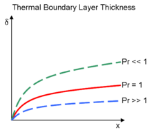
Plot showing the relative thickness in the Thermal boundary layer versus the Velocity boundary layer (in red) for various Prandtl Numbers. For Pr=1{displaystyle Pr=1}, the two are equal.

δδT=Pr1/3{displaystyle {delta over delta _{T}}=Pr^{1/3}}          and therefore          δδc=Sc1/3{displaystyle {delta over delta _{c}}=Sc^{1/3}}

From this solution, it is possible to characterize the convective heat/mass transfer constants based on the region of boundary layer flow. Fourier’s law of conduction and Newton’s Law of Cooling are combined with the flux term derived above and the boundary layer thickness.

qA=−k(∂T∂y)y=0=hx(TS−T∞){displaystyle {q over A}=-kleft({partial T over partial y}right)_{y=0}=h_{x}(T_{S}-T_{infty })}

hx=0.332kxRex1/2Pr1/3{displaystyle h_{x}=0.332{k over x}Re_{x}^{1/2}Pr^{1/3}}

This gives the local convective constant hx{displaystyle h_{x}} at one point on the semi-infinite plane. Integrating over the length of the plate gives an average

hL=0.664kxReL1/2Pr1/3{displaystyle h_{L}=0.664{k over x}Re_{L}^{1/2}Pr^{1/3}}

Following the derivation with mass transfer terms (k{displaystyle k} = convective mass transfer constant, DAB{displaystyle D_{AB}} = diffusivity of species A into species B, Sc=ν/DAB{displaystyle Sc=nu /D_{AB}} ), the following solutions are obtained:

kx′=0.332DABxRex1/2Sc1/3{displaystyle k'_{x}=0.332{D_{AB} over x}Re_{x}^{1/2}Sc^{1/3}}

kL′=0.664DABxReL1/2Sc1/3{displaystyle k'_{L}=0.664{D_{AB} over x}Re_{L}^{1/2}Sc^{1/3}}

These solutions apply for laminar flow with a Prandtl/Schmidt number greater than 0.6.^[22]

Naval architecture

Many of the principles that apply to aircraft also apply to ships, submarines, and offshore platforms.

For ships, unlike aircraft, one deals with incompressible flows, where change in water density is negligible (a pressure rise close to 1000kPa leads to a change of only 2–3 kg/m³). This field of fluid dynamics is called hydrodynamics. A ship engineer designs for hydrodynamics first, and for strength only later. The boundary layer development, breakdown, and separation become critical because the high viscosity of water produces high shear stresses. Another consequence of high viscosity is the slip stream effect, in which the ship moves like a spear tearing through a sponge at high velocity.^{[citation needed]}

Boundary layer turbine

This effect was exploited in the Tesla turbine, patented by Nikola Tesla in 1913. It is referred to as a bladeless turbine because it uses the boundary layer effect and not a fluid impinging upon the blades as in a conventional turbine. Boundary layer turbines are also known as cohesion-type turbine, bladeless turbine, and Prandtl layer turbine (after Ludwig Prandtl).

Predicting Transient Boundary Layer Thickness in a Cylinder Using Dimensional Analysis

By using the transient and viscous force equations for a cylindrical flow you can predict the transient boundary layer thickness by finding the Womersley Number (Nw{displaystyle N_{w}}).

Transient Force = ρvw{displaystyle rho vw}

Viscous Force = μvδ12{displaystyle {mu v over delta _{1}^{2}}}

Setting them equal to each other gives:

ρvw=μvδ12{displaystyle rho vw={mu v over delta _{1}^{2}}}

Solving for delta gives:

δ1=μρw= v w{displaystyle delta _{1}={sqrt {mu over rho w}}={sqrt { v over w}}}

In dimensionless form:

Lδ1=Lw v=Nw{displaystyle {L over delta _{1}}={L{sqrt {w over v}}}=N_{w}}

Where Nw{displaystyle N_{w}} = Womersley Number; ρ{displaystyle rho } = density; v{displaystyle v} = velocity; w={displaystyle w=} ?; δ1{displaystyle delta _{1}} = length of transient boundary layer; μ{displaystyle mu } = viscosity; L{displaystyle L} = characteristic length.

Predicting Convective Flow Conditions at the Boundary Layer in a Cylinder Using Dimensional Analysis

By using the convective and viscous force equations at the boundary layer for a cylindrical flow you can predict the convective flow conditions at the boundary layer by finding the dimensionless Reynolds Number (NR{displaystyle N_{R}}).

Convective Force = ρv2 L{displaystyle rho v^{2} over L}

Viscous Force = μvδ22{displaystyle {mu v over delta _{2}^{2}}}

Setting them equal to each other gives:

ρv2 L=μvδ22{displaystyle {rho v^{2} over L}={mu v over delta _{2}^{2}}}

Solving for delta gives:

δ2=μLρv{displaystyle delta _{2}={sqrt {mu L over rho v}}}

In dimensionless form:

Lδ2=ρvLμ=NR{displaystyle {L over delta _{2}}={sqrt {rho vL over mu }}={sqrt {N_{R}}}}

Where NR{displaystyle N_{R}} = Reynolds Number; ρ{displaystyle rho } = density; v{displaystyle v} = velocity; δ2{displaystyle delta _{2}} = length of convective boundary layer; μ{displaystyle mu } = viscosity; L{displaystyle L} = characteristic length.

Boundary layer ingestion

Boundary layer ingestion promises an increase in aircraft fuel efficiency with an aft-mounted propulsor ingesting the slow fuselage boundary layer and re-energising the wake to reduce drag and improve propulsive efficiency.
To operate in distorted airflow, the fan is heavier and its efficiency is reduced, and its integration is challenging.
It is used in concepts like the Aurora D8 or the French research agency Onera’s Nova, saving 5% in cruise by ingesting 40% of the fuselage boundary layer.^[24]

Airbus presented the Nautilius concept at the ICAS congress in September 2018:
to ingest all the fuselage boundary layer, while minimizing the azimuthal flow distortion, the fuselage splits into two spindles with 13-18:1 bypass ratio fans.
Propulsive efficiencies are up to 90% like counter-rotating open rotors with smaller, lighter, less complex and noisy engines.
It could lower fuel burn by over 10% compared to an usual underwing 15:1 bypass ratio engine.^[24]

See also

• Boundary layer separation


• Boundary-layer thickness


• Thermal boundary layer thickness and shape


• Boundary layer suction


• Boundary layer control


• Blasius boundary layer


• Falkner–Skan boundary layer


• Ekman layer


• Planetary boundary layer


• Logarithmic law of the wall


• Shape factor (boundary layer flow)


• Shear stress

References

• 
  Chanson, H. (2009). Applied Hydrodynamics: An Introduction to Ideal and Real Fluid Flows. CRC Press, Taylor & Francis Group, Leiden, The Netherlands, 478 pages. ISBN 978-0-415-49271-3.
  


• A.D. Polyanin and V.F. Zaitsev, Handbook of Nonlinear Partial Differential Equations, Chapman & Hall/CRC Press, Boca Raton – London, 2004.
  ISBN 1-58488-355-3
  


• A.D. Polyanin, A.M. Kutepov, A.V. Vyazmin, and D.A. Kazenin, Hydrodynamics, Mass and Heat Transfer in Chemical Engineering, Taylor & Francis, London, 2002.
  ISBN 0-415-27237-8
  


• Hermann Schlichting, Klaus Gersten, E. Krause, H. Jr. Oertel, C. Mayes "Boundary-Layer Theory" 8th edition Springer 2004
  ISBN 3-540-66270-7
  


• John D. Anderson, Jr., "Ludwig Prandtl's Boundary Layer", Physics Today, December 2005


• 
  Anderson, John (1992). Fundamentals of Aerodynamics (2nd ed.). Toronto: S.S.CHAND. pp. 711–714. ISBN 0-07-001679-8.
  


• 
  H. Tennekes and J. L. Lumley, "A First Course in Turbulence", The MIT Press, (1972).


• Lectures in Turbulence for the 21st Century by William K. George

External links

• National Science Digital Library – Boundary Layer


• Moore, Franklin K., "Displacement effect of a three-dimensional boundary layer". NACA Report 1124, 1953.


• Benson, Tom, "Boundary layer". NASA Glenn Learning Technologies.


• Boundary layer separation


• 
  Boundary layer equations: Exact Solutions – from EqWorld


• Jones, T.V. BOUNDARY LAYER HEAT TRANSFER

References

^ Young, A.D. (1989). Boundary layers (1st publ. ed.). Washington, DC: American Institute of Aeronautics and Astronautics. ISBN 0930403576..mw-parser-output cite.citation{font-style:inherit}.mw-parser-output q{quotes:"""""""'""'"}.mw-parser-output code.cs1-code{color:inherit;background:inherit;border:inherit;padding:inherit}.mw-parser-output .cs1-lock-free a{background:url("//upload.wikimedia.org/wikipedia/commons/thumb/6/65/Lock-green.svg/9px-Lock-green.svg.png")no-repeat;background-position:right .1em center}.mw-parser-output .cs1-lock-limited a,.mw-parser-output .cs1-lock-registration a{background:url("//upload.wikimedia.org/wikipedia/commons/thumb/d/d6/Lock-gray-alt-2.svg/9px-Lock-gray-alt-2.svg.png")no-repeat;background-position:right .1em center}.mw-parser-output .cs1-lock-subscription a{background:url("//upload.wikimedia.org/wikipedia/commons/thumb/a/aa/Lock-red-alt-2.svg/9px-Lock-red-alt-2.svg.png")no-repeat;background-position:right .1em center}.mw-parser-output .cs1-subscription,.mw-parser-output .cs1-registration{color:#555}.mw-parser-output .cs1-subscription span,.mw-parser-output .cs1-registration span{border-bottom:1px dotted;cursor:help}.mw-parser-output .cs1-hidden-error{display:none;font-size:100%}.mw-parser-output .cs1-visible-error{font-size:100%}.mw-parser-output .cs1-subscription,.mw-parser-output .cs1-registration,.mw-parser-output .cs1-format{font-size:95%}.mw-parser-output .cs1-kern-left,.mw-parser-output .cs1-kern-wl-left{padding-left:0.2em}.mw-parser-output .cs1-kern-right,.mw-parser-output .cs1-kern-wl-right{padding-right:0.2em}
^ Prandtl, L. "Zur berechnung der grenzschichten." ZAMM‐Journal of Applied Mathematics and Mechanics/Zeitschrift für Angewandte Mathematik und Mechanik 18.1 (1938): 77-82.
^ Van Dyke, Milton. Perturbation methods in fluid mechanics. Parabolic Press, Incorporated, 1975.
^ Stewartson, K. "On asymptotic expansions in the theory of boundary layers." Studies in Applied Mathematics 36.1-4 (1957): 173-191.
^ Libby, Paul A., and Herbert Fox. "Some perturbation solutions in laminar boundary-layer theory." Journal of Fluid Mechanics 17.03 (1963): 433-449.
^ Fox, Herbert, and Paul A. Libby. "Some perturbation solutions in laminar boundary layer theory Part 2. The energy equation." Journal of Fluid Mechanics 19.03 (1964): 433-451.
^ Kármán, Th V. "Über laminare und turbulente Reibung." ZAMM‐Journal of Applied Mathematics and Mechanics/Zeitschrift für Angewandte Mathematik und Mechanik 1.4 (1921): 233-252.
^ Wieghardt, K. On an energy equation for the calculation of laminar boundary layers. Joint Intelligence Objectives Agency, 1946.
^ Wieghardt, Karl. "über einen Energiesatz zur Berechnung laminarer Grenzschichten." Ingenieur-Archiv 16.3-4 (1948): 231-242.
^ Rosenhead, Louis, ed. Laminar boundary layers. Clarendon Press, 1963.
^ Von Mises, Richard. "Bemerkungen zur hydrodynamik." Z. Angew. Math. Mech 7 (1927): 425-429
^ Karman. "T. von & Tsien, HS." J. Aero. Sci. 1938 (1938): 5-227.
^ Crocco, L. "A characteristic transformation of the equations of the boundary layer in gases." ARC 4582 (1939): 1940.
^ Lévêque, A. (1928). "Les lois de la transmission de chaleur par convection". Annales des Mines ou Recueil de Mémoires sur l'Exploitation des Mines et sur les Sciences et les Arts qui s'y Rattachent, Mémoires (in French). XIII (13): 201–239.
^ ab Niall McMahon. "André Lévêque p285, a review of his velocity profile approximation". Archived from the original on 2012-06-04.
^ ab Martin, H. (2002). "The generalized Lévêque equation and its practical use for the prediction of heat and mass transfer rates from pressure drop". Chemical Engineering Science. 57 (16). pp. 3217–3223. doi:10.1016/S0009-2509(02)00194-X.
^ Schuh, H. (1953). "On asymptotic solutions for the heat transfer at varying wall temperatures in a laminar boundary layer with Hartree's velocity profiles". Jour. Aero. Sci. 20 (2). pp. 146–147.
^ Kestin, J. & Persen, L.N. (1962). "The transfer of heat across a turbulent boundary layer at very high prandtl numbers". Int. J. Heat Mass Transfer. 5: 355–371. doi:10.1016/0017-9310(62)90026-1.
^ Schlichting, H. (1979). Boundary-Layer Theory (7 ed.). New York (USA): McGraw-Hill.
^ Blasius, H. (1908). "Grenzschichten in Flüssigkeiten mit kleiner Reibung". Z. Math. Phys. 56: 1–37. (English translation)
^ Martin, Michael J. Blasius boundary layer solution with slip flow conditions. AIP conference proceedings 585.1 2001: 518-523. American Institute of Physics. 24 Apr 2013.
^ ab Geankoplis, Christie J. Transport Processes and Separation Process Principles: (includes Unit Operations). Fourth ed. Upper Saddle River, NJ: Prentice Hall Professional Technical Reference, 2003. Print.
^ Pohlhausen, E. (1921), Der Wärmeaustausch zwischen festen Körpern und Flüssigkeiten mit kleiner reibung und kleiner Wärmeleitung. Z. angew. Math. Mech., 1: 115–121. doi:10.1002/zamm.19210010205
^ ab Graham Warwick (Nov 19, 2018). "The Week In Technology, November 19-23, 2018". Aviation Week & Space Technology.